Improving treatment effect estimates with multivariate adaptive shrinkage (mashr)

An illustrative example

In this post I illustrate the utility of mashr in a simple case where we have two outcomes of interest (metric a and metric b) and their corresponding observed treatment effects for many A/A experiments – that is, where there is actually no true experimental effects at all. This will help demonstrate the problem of correlated sampling error and how mashr helps address it.

First let’s start by simulating two standard normal metrics – a and b – with a unit level correlation of 0.40:

set.seed(1)

# set sample size
N <- 1000000

# define two standard normal variables with a correlation of r = 0.40
data_matrix <- mvrnorm(
    n = N, 
    mu = c(0, 0), 
    Sigma = matrix(c(1, .4, .4, 1), nrow = 2), 
    empirical = TRUE
)

df <- tibble(
    id = 1:N,
    a = data_matrix[, 1],
    b = data_matrix[, 2]
)

# confirm unit level correlation of 0.4
df %>% summarise(correlation = cor(a, b))
## # A tibble: 1 × 1
##   correlation
##         <dbl>
## 1         0.4

Next let’s simulate 1000 A/A tests by randomly assigning people to treatment or control groups:

df <- df %>%
    mutate(
        # randomly assign participants to a treatment or control condition (i.e., a/a test)
        condition = if_else(
            rbinom(N, 1, .5) == 0, 
            "control", 
            "treatment"
        ),
        # split into 1000 groups
        experiment = id %% 1000
    )

Finally we can calculate the 1k observed treatment effects for metric a and metric b:

# set critical value
alpha_level <- 0.05
confidence_level <- 1 - alpha_level
critical_value <- qnorm(1 - alpha_level / 2)

# calculate observed treatment effects
treatment_effects <- df %>% 
    pivot_longer(
        cols = c(a, b), 
        names_to = "measure", 
        values_to = "value"
    ) %>%
    group_by(experiment, condition, measure) %>%
    summarise(
        mean = mean(value),
        se = sd(value) / sqrt(n())
    ) %>%
    ungroup() %>%
    pivot_wider(
        names_from = c(condition, measure),
        values_from = c(mean, se)
    ) %>%
    mutate(
        a_delta = mean_treatment_a - mean_control_a,
        a_delta_se = sqrt(se_treatment_a^2 + se_control_a^2),
        a_delta_moe = a_delta_se * critical_value,
        a_delta_conf.low = a_delta - a_delta_moe,
        a_delta_conf.high = a_delta + a_delta_moe,
        a_delta_is_sig = if_else(
            a_delta_conf.low > 0 | a_delta_conf.high < 0,
            1,
            0
        ),
        b_delta = mean_treatment_b - mean_control_b,
        b_delta_se = sqrt(se_treatment_b^2 + se_control_b^2),
        b_delta_moe = b_delta_se * critical_value,
        b_delta_conf.low = b_delta - b_delta_moe,
        b_delta_conf.high = b_delta + b_delta_moe,
        b_delta_is_sig = if_else(
            b_delta_conf.low > 0 | b_delta_conf.high < 0,
            1,
            0
        ),
    )

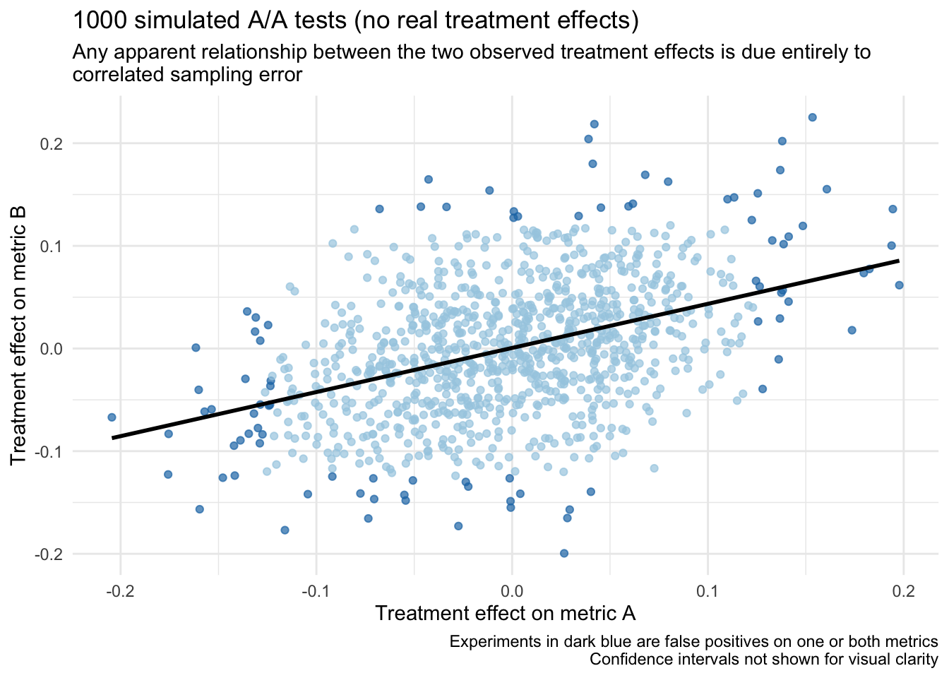
What do we observe? As expected, we observe a false positive rate of around 5% for each metric. But more importantly, recall that the unit level correlation between metrics a and b is r = 0.40. Now, even though there are no “real” treatment effects in any of these experiments (i.e., they are all A/A tests), we still expect to observe a correlation among the treatment effects around this same value (i.e., r = 0.40) due to correlated sampling error.

# look at correlation of treatment effects and frequency of false positives
treatment_effects %>% summarise(
    delta_correlation = cor(a_delta, b_delta),
    a_delta_false_positive = mean(a_delta_is_sig),
    b_delta_false_positive = mean(b_delta_is_sig)
    )
## # A tibble: 1 × 3
##   delta_correlation a_delta_false_positive b_delta_false_positive
##               <dbl>                  <dbl>                  <dbl>
## 1             0.414                  0.053                   0.05

To help drive this point home, if we look at a scatter plot of these treatment effects (w/ a regression line) it looks like there could be a relationship, but it is actually entirely a result of sampling error:

Given that we know the “real” treatment effect for all of these experiments is actually 0, what can we do to get better estimates?

Apply multivariate adaptive shrinkage (mashr).

Applying mashr

The mashr R package (see Urbut et al., 2019) implements the multivariate adaptive shrinkage method.

At its core, all we need to provide mashr is a matrix of the observed treatment effect estimates (Bhat) and a corresponding matrix of the standard errors of those treatment effect estimates (Shat):

Bhat <- treatment_effects %>%
    select(
        a_delta,
        b_delta
    ) %>%
    as.matrix()

Shat <- treatment_effects %>%
    select(
        a_delta_se,
        b_delta_se
    ) %>%
    as.matrix()

mashr_data <- mash_set_data(Bhat, Shat)

In settings where the outcome measurements are correlated with each other (like ours), mashr also provides a method to incorporate this information to help reduce false positives. Specifically, we can use an estimate of the correlation in treatment effects among null experiments:

null_correlations <- estimate_null_correlation_simple(mashr_data)
null_correlations
##           a_delta   b_delta
## a_delta 1.0000000 0.3391389
## b_delta 0.3391389 1.0000000

And then we can update our mashr data object with this information:

mashr_data_w_correlations <- mash_update_data(mashr_data, V = null_correlations)

Finally, we create a set of covariance matrices that mashr will use to fit the model. The estimated mixture proportions assigned to each of these matrices will help us determine which is most consistent with the data. mashr provides methods for both “canonical” and “data driven” covariance matrices, and here we’ll just use the canonical matrices:

• Identity matrix: Effects are independent among conditions
• Singleton matrices: Effects are specific to a given metric (a or b) only
• Equal effects matrix: Effects are equal for both metrics
• Simple het matrices: Effects are correlated to varying degrees

# specify the canonical covariance matrices
U.c <- cov_canonical(mashr_data_w_correlations) 

Now we can fit the model!

mashr_results <- mash(mashr_data_w_correlations, U.c) 
##  - Computing 1000 x 99 likelihood matrix.
##  - Likelihood calculations took 0.05 seconds.
##  - Fitting model with 99 mixture components.
##  - Model fitting took 0.17 seconds.
##  - Computing posterior matrices.
##  - Computation allocated took 0.01 seconds.

mashr then provides a series of very useful functions to extract relevant information from the model.

For example, we can get the improved posterior treatment effect estimates and their corresponding standard errors (which we could choose to visualize in a plot):

# get posterior means
head(get_pm(mashr_results) %>% as_tibble())
## # A tibble: 6 × 2
##     a_delta   b_delta
##       <dbl>     <dbl>
## 1 -0.00467  -0.00467 
## 2  0.00317   0.00317 
## 3 -0.00156  -0.00156 
## 4 -0.000484 -0.000484
## 5  0.00163   0.00163 
## 6 -0.00221  -0.00221

# get posterior SDs
head(get_psd(mashr_results) %>% as_tibble())
## # A tibble: 6 × 2
##   a_delta b_delta
##     <dbl>   <dbl>
## 1 0.0187  0.0187 
## 2 0.0153  0.0153 
## 3 0.0108  0.0108 
## 4 0.00752 0.00752
## 5 0.0110  0.0110 
## 6 0.0127  0.0127

Or we can find experiments where the improved posterior treatment effect estimate is statistically significant in at least one condition.

Note: we find no “significant” conditions here because mashr has (correctly!) learned that most experiments are null and shrunk the treatment effect estimates toward 0

# get effects that are significant in at least one condition
get_significant_results(mashr_results)
## integer(0)

Understanding how often two treatment effects share effects is particularly useful for evaluating the utility of a potential “proxy” or “surrogate” metric for another metric that is more expensive or difficult to measure (e.g., if my proxy candidate moves, how often does my ground truth metric of interest also move at least in the same direction but ideally also within a similar magnitude?).

Note: we again find no relevant signals here because mashr has correctly identified that there are actually no “real” treatment effects in these experiments… but these functions are very useful in applied use cases.

# get the proportion of (significant) signals shared by some specified magnitude
get_pairwise_sharing(mashr_results, factor = 0.5)
##         a_delta b_delta
## a_delta     NaN     NaN
## b_delta     NaN     NaN

# get the proportion of (significant) signals that at least share the same sign
get_pairwise_sharing(mashr_results, factor = 0)
##         a_delta b_delta
## a_delta     NaN     NaN
## b_delta     NaN     NaN

Finally we can look at the mixture proportions for the different types of covariance matrices used in the modeling. This is very useful to understand which covariance matrices are most consistent with the observed data (where in this case the model correctly assigns the overwhelming majority of the weight to the null covariance matrix, meaning the data is most consistent with entirely null effects):

# get the estimated mixture proportions
get_estimated_pi(mashr_results)
##          null      identity       a_delta       b_delta equal_effects 
##    0.95480945    0.00000000    0.00000000    0.00000000    0.04519055 
##  simple_het_1  simple_het_2  simple_het_3 
##    0.00000000    0.00000000    0.00000000

Takeaway

Any time we have observed treatment effects on multiple outcomes – here we just used two outcomes but in practice we could have many, many more! – multivariate adaptive shrinkage (mashr) is an extremely valuable tool for deriving improved (posterior) treatment effect estimates for all of them by leveraging all the shared information across experiments.

mashr is also particularly useful when evaluating the utility of a “proxy” or “surrogate” metric, because it will result in better estimates of how often the proxy vs. ground truth treatment effects actually correspond with each other in direction and/or magnitude.

Note: full R Markdown used for this post is available @ https://github.com/ryansritter/mashr_intro